Part 4 – Testing with Simulated Timing

prev

Everything we’ve looked at so far has disregarded any propagation delay. While trying to achieve the correct logic, this is reasonable. However, there will come a point where a design has to be synthesised, and propagation delay effects cannot be ignored.

Delays introduce significant risks, such as hazards and (in the case of synchronous systems) missed deadlines such as set-up or hold time violations. VHDL has a facility to model propagation delay. In practise, gate delays will depend on the type of FPGA and the routing. We use the synthesis tools in Quartus to generate these for us.

To help us understand how delays are modelled in VHDL, we will begin by assuming known values for delays in each component. In the next section, we will use Quartus to do this for a real design.

Modelling Delay

For illustrative purposes, we will assume the following timing characteristics:

• INVERTER – 5ns
• OR gate – 10ns
• AND gate – 10ns

Let’s not update both architectures in comp1 to model these delays.

library ieee;				
use ieee.std_logic_1164.all;
--use ieee.std_logic_unsigned.all;

-- Component 1 - very simple device that performs a logical OR on three single bit inputs
entity comp1 is
port(  	A:	in std_logic;
	B:	in std_logic;
	C:	in std_logic;
	Y:	out std_logic
);
end comp1;

--This component has two architecture
architecture v1 of comp1 is
begin
	y <= A or B or C after 10 ns;
end v1;

--This second version is supposed to be functionally equivalent
--Bug squashed!
architecture v2 of comp1 is
	signal notA, notB, notC : std_logic;
	signal or3 : std_logic;
begin
--	y <= ((not A) and (not B) and  (not C));
	notA <= not A after 5 ns;
	notB <= not B after 5 ns;
	notC <= not C after 5 ns;
	or3  <= (notA and notB and notC) after 10 ns;
	y    <= not or3 after 5 ns;
end v2;

This is mostly self-explanatory. The after keyword is used by the simulator (and ignored during synthesis) to add delays to signal changes.

Note the following:

• The first architecture is clearly going to be faster – however, in more complex systems, this may not be so obvious for all input combinations and sequences.
• The second architecture is broken down for clarity. This could have been written in one line, but it would be very difficult to read and debug.

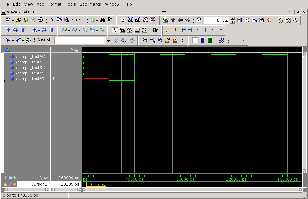
Let’s now examine the simulation output using ModelSim:

It is clear from the figure above that the second architecture has longer propagation delay from input to output.

Checking Timing with a Test Bench

Let’s modify the testbench to make allowances for timing.The delay will also be removed from the first architecture so it acts as a perfect reference. Our intention is that the second architecture will have the correct output within 15ns.

--Exhaustive test
for idx in 0 to 7 loop
	--Convert integer idx to std_logic
	count := std_logic_vector(to_unsigned(idx,3));

	--Assign internal signals to the individual bits of count
	AA <= count(0);
	BB <= count(1);
	CC <= count(2);

	--Looking for differences in the output
	wait for 5 ns;
	assert(Y1 = Y2) report "Mismatch at 5ns" severity warning;
	wait for 5 ns;
	assert(Y1 = Y2) report "Mismatch at 10ns" severity warning;
	wait for 5 ns;
	assert(Y1 = Y2) report "Mismatch at 15ns" severity error;
	wait for 5 ns;
	assert(Y1 = Y2) report "Mismatch at 20ns" severity error;
end loop;

Note the following:

• the input signals are changed every 20ns (4 x 5ns)
• we are assuming architecture 1 is a perfect benchmark for the second. This is only possible because we are simulating
• the different severity types (error is a failure)
• we have covered all combinations, but not all possible sequences of input (e.g. 000->111)

The test output is shown as follows:

run -all
# ** Warning: Mismatch at 5ns
#    Time: 5 ns  Iteration: 0  Instance: /comp1_test
# ** Warning: Mismatch at 10ns
#    Time: 10 ns  Iteration: 0  Instance: /comp1_test
# ** Error: Mismatch at 15ns
#    Time: 15 ns  Iteration: 0  Instance: /comp1_test
# ** Warning: Mismatch at 5ns
#    Time: 25 ns  Iteration: 0  Instance: /comp1_test
# ** Warning: Mismatch at 10ns
#    Time: 30 ns  Iteration: 0  Instance: /comp1_test
# ** Error: Mismatch at 15ns
#    Time: 35 ns  Iteration: 0  Instance: /comp1_test

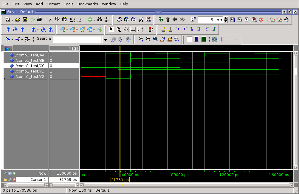
The highlighted lines are errors, failing at 15ns and 35ns. We can see this from the ModelSim waveform output:

An obvious limitation with this approach is the assumed propagation delays. In the next section, we will use Quartus to more accurately simulate real delays on a specific FPGA.

Next – Part 5 – Timing Checks