Pulse Width Modulation (PWM) – (Glossary Entry)

Pulse Width Modulation is a technique of generating a digital pulse that delivers a controllable amount of power. For example, if we wish to control a DC motor, then the amount of power delivered to the motor will dictate the motor speed. Equally, if controlling an LED, the power delivered will determine the brightness.
Consider the digital waveform below:

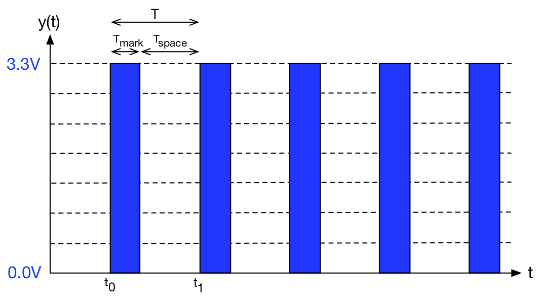
Illustrating the output from a Pulse Width Modulation (PWM) process

The digital pulse of ‘1’ is represented by the blue regions.

The output is a ON for $T_{mark}$ seconds and off for $T_{space}$ seconds and that $T = T_{mark}+T_{space}$ . If this signal is driving a device such as an LED or a DC motor, then clearly $T$ needs to be kept small to avoid noticeable pulsing effects (although for motors, $T$ must not be too small as you will discover).

The ratio of time spend ON, that is $\frac{T_{mark}}{T}$ is known as the duty cycle. Often this is expressed as a percentage, so $duty = \frac{T_{mark}}{T} \cdot 100 \%$

Intuition would suggest the average output voltage is somehow related to the proportion of time that the output is ON. Let’s look at this more formally.

In general, for a voltage signal $v(t)$ that varies with time $t$ , we can say that the mean voltage $\overline{v(t)}$ is derived as

$\overline{v(t)} = \frac{1}{T} \cdot \int_{t_0}^{t_1} v(t) dt$

However, from the graph, $v(t)$ is a constant over fixed durations, so we can split this up and exploit this. We say that

$\overline{v(t)} = \frac{1}{T} \cdot \int_{t_0}^{t_0 + t_{mark}} V dt + \frac{1}{T} \cdot \int_{t_0+t_{mark}}^{t_1} 0 dt$

where $V=3.3V$ . The integral of zero is always zero, so we can write

$\overline{v(t)} = \frac{V}{T} \cdot \int_{t_0}^{t_0 + t_{mark}} 1 dt + 0$

Integrating, we get

$\overline{v(t)} = \frac{V}{T} \cdot \left[ t \right]_{t_0}^{t_0 + T_{mark}}$

$\overline{V(t)} =\frac{V}{T}\cdot\left[ t_0+T_{mark}-t_0 \right]$

$\overline{V(t)} =\frac{T_{mark}}{T} \cdot V$

Intuition would also suggest the output power is somehow related to the proportion of time that the output is ON. Let’s look at this more formally.

Consider driving power into a load resistance of $R \Omega$ , the instantaneous power is calculated as $P(t)=\frac{v(t)^2}{R}$ . What is more useful is the mean power over a period of time. It is therefore the mean of $v(t)^2$ that is of interest. As $V$ and $R$ are constants, by the same reasoning

$\overline{P(t)} =\frac{T_{mark}}{T} \cdot \frac{V^2}{R}$

In summary, we can rewrite both these equations as follows:

$mean\ voltage=\frac{T_{mark}}{T_{mark}+T_{space}}\cdot V$

$mean\ power=\frac{T_{mark}}{T_{mark}+T_{space}}\cdot \frac{V^2}{R}$

Practical Application

Consider a DC motor. Put simply, we are turning the motor on and off at a fixed frequency. If $T=1s$ , then you would see the motor starting and stopping, causing a juddering. The fundamental frequency of the vibration is $f_{0}=1/T \ Hz$ .

If $f_{0}$ is in the audible spectrum ( $<20kHz$ ), it will make the motor noisier.
However, if $f_{0}$ is too high, the “inductive” effects of the motor will significantly reduce the power delivered to the motor (the details of this is something you will study later in the course).

As is often the case in engineering, you have to balance trade-offs between different criteria.For now, we are going to do this ‘empirically’.