In this section we look at interfacing with the analogue world. You will use a simple potentiometer to generate analogue voltages, and measure that voltage using an Analogue to Digital Converter (ADC). We also look at different ways to represent an analogue voltage as a digital value. Hysteresis is used to manage signal noise and avoid output jitter. You will also discover problems with noise, and use ‘hysteresis’ to avoid instability due to noise.

Intended Learning Outcomes

Use a potentiometer to generate and control an analogue signal
Convert an analogue signal to an integer digital representation using an analogue to digital converter
Scale an integer value to a fractional value
Use hysteresis thresholds to avoid problems with noise
Use conditional statements and operators to make decisions in software
Break a program into logical and reusable functions
Use looping commands to perform iteration to average a measurement
Use a hardware interrupt timer for accurate sampling.

Activity 4.1 Potentiometer

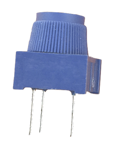
In this section, we are going to use a “potentiometer” to create an analogue signal. Your potentiometer should look something like the figure below.

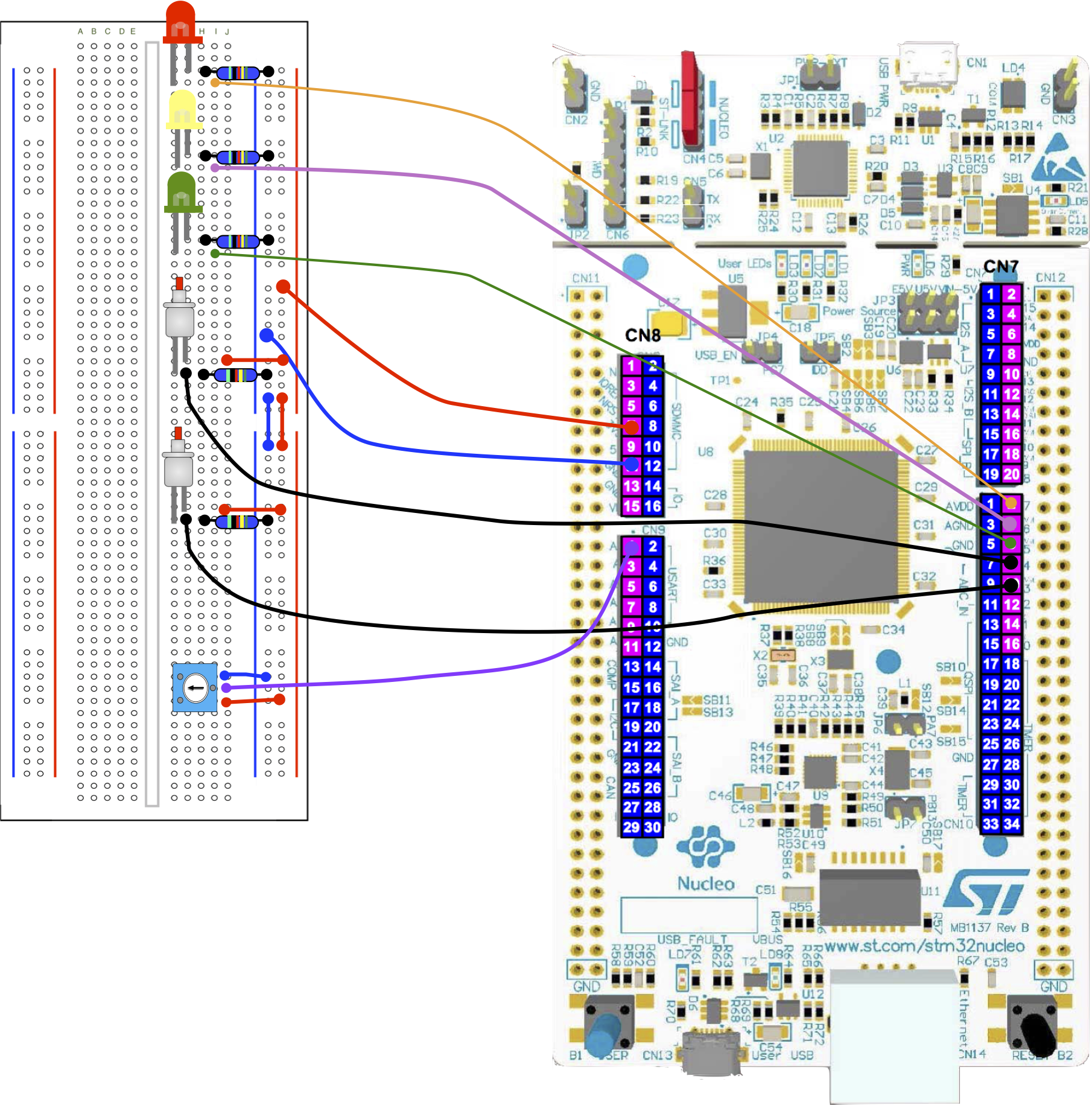
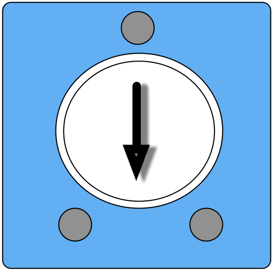
Photo of the Potentiometer used in this course

Below is a diagram for the prototype board. We have simply added a potentiometer to the circuit, with the middle terminal connected to pin A0.

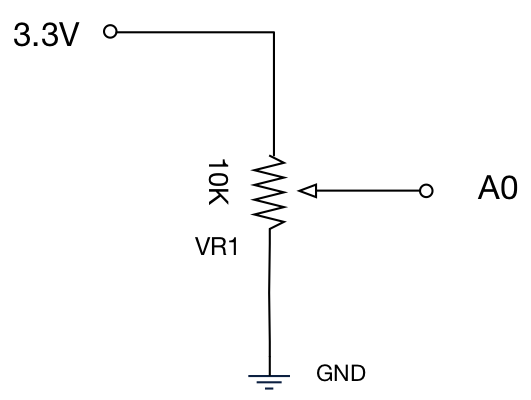
The prototyping board layout is shown above. Note the power supply rails have been linked to extended the power rails.

The schematic for the potentiometer is shown below.

Potentiometer Circuit schematic, providing a variable voltage input to the analogue input A0

(unofficial) Symbol for the potentiometer for prototyping diagrams

Task 4.1.1

Perform the following steps:

Wire the circuit shown. Instead of connecting the wire to A0, connect it to a DVM on the voltage range.

By rotating the potentiometer (POT), what range of voltages do you observe?

Now connect the center terminal wire to A0 (as shown in the figure above)

Create new project, paste in the code below, compile and and run.

Run the terminal (PuTTY) to see the output. If nothing appears, you may need to change the COM port setting (use Windows Device Manager to check)

Set the POT to the two extremes and observe the values

Set the POT such that you get close to 0.5.

Are you able to get precisely 0.5, and if not, why?

Using an if-else statement, write some additional code to switch the Green LED ON when the analogue input is between 0.0 and 0.5, the Red LED ON when greater than 0.5 and 1.0. A solution is available here. See the glossary entry about if-else if-else if you are unsure.

Set the POT to halfway, and try and make the LED’s switch on and off erratically.

Sometimes we might write the specification as follows:

$colour = \left\{ \begin{array}{ll} GREEN & V_{in}<0.5 \\ RED & otherwise$

#include "mbed.h"

//Global objects
BusOut binaryOutput(D5, D6, D7);    
DigitalIn SW1(D3);
DigitalIn SW2(D4);

//Analog input
AnalogIn AIN(A0);

//Global variable
float fVin = 0.0;

//Main function
int main() {
    
    while(1) {
        
        //Read ADC
        fVin = AIN;
        
        //Write to terminal
        printf("Analog input = %5.3f\n", fVin); 
        
        //Wait
        wait(0.5);
        
    } //end while(1)
} //end main

AnalogIn

In this example we introduce the Mbed-os type AnalogIn. This enables use to access an on-chip analogue to digital converter that converts an analogue signal to a digital representation. We create a variable of type AnalogIn much like we did with DigitalIn :

AnalogIn AIN(A0);

Like DigitalIn , the single parameter is the pin name A0. We read the analogue input value as follows:

fVin = AIN;

Note the data type of fVin is float. This type of data can hold fractional numbers, as opposed the int and unsigned int data types that only hold whole numbers. Using this method, the value we read is conveniently scaled between 0.0 (0V) and 1.0 (3.3V).

Observations

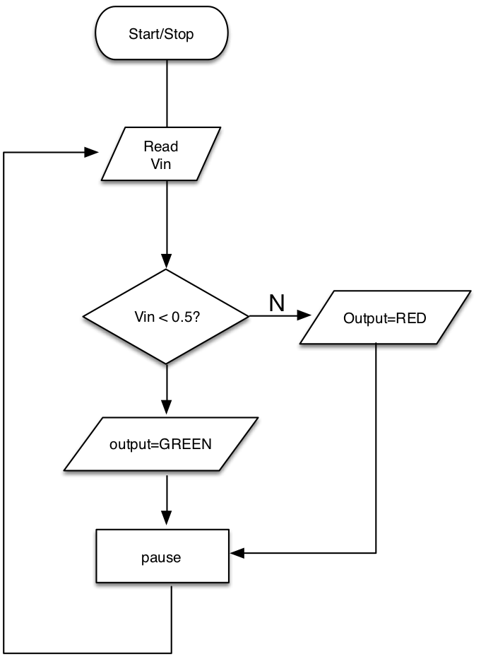
No signals are ever perfectly constant. The observed value we see changes due to electrical noise. Noise is always present, so as the value gets close to 0.5, there will always be some point where the output “jitters” between RED to GREEN. The output is unstable at this point.

Consider the case where the output is not an LED, but something more critical:

lift motor – In such states, it will stop and start erratically, possibly causing damage, passenger discomfort and undue mechanical wear.
automatic defibrillator – a device to inject a unit of energy across a human chest to reset the electrical characteristics of the heart and hopefully restore its rhythm. You would certainly not want erratic outputs for such a device!

Noise is not the only problem, as over longer periods of time, other factors such as temperature changes and component ageing can cause component values to drift. We will address these problems using hysteresis in a later task.

Task 4.1.2

Complete the following:

The flow chart below is for Task 4.1.1 (previous task). Sketch a new flow chart to use three LEDs, as specified by the equation

$colour = \left\{ \begin{array}{ll} GREEN & 0.0 \leq V_{in} < 0.4 \\ YELLOW & 0.4 \leq V_{in} < 0.6 \\ GREEN & otherwise$

Again, using if, else if and else statements, code your solution and test.

Does it still have regions when outputs are unstable?

A solution is given here.

Flow-chart for the simple threshold detector. Note this design suffers from output jitter in the region around Vin=0.5

Task 4.1.3

Perform the following tasks:

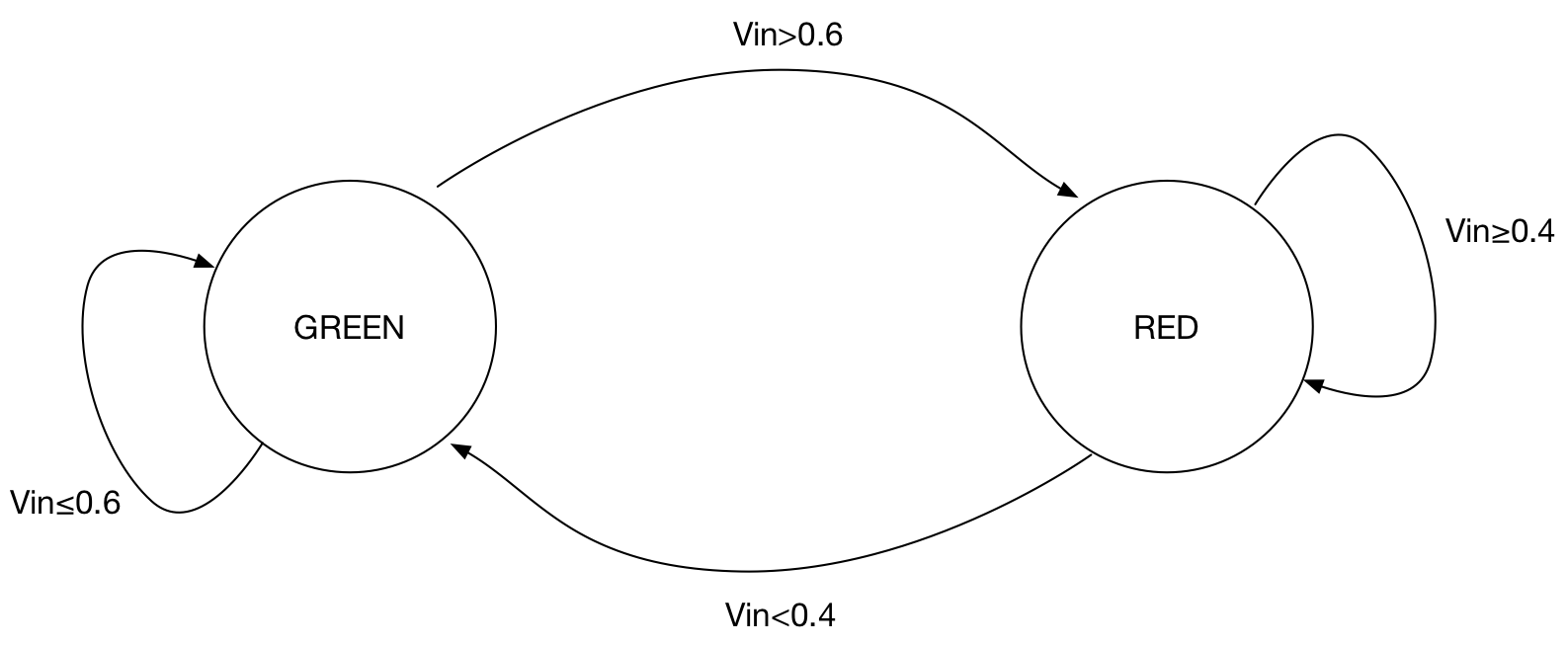
The code below uses hysteresis to avoid the problem of noise for a single threshold.

Read the glossary entry on Hysteresis

Question: what is the noise margin?

Sketch a flow chart for this code

#include "mbed.h"


#define kRED    (1 << 2)    //4
#define kYELLOW (1 << 1)    //2
#define kGREEN  (1 << 0)    //1

//Global objects
//Outputs as an integer
BusOut binaryOutput(D5, D6, D7);    

//Analogue Input
AnalogIn AIN(A0);
float fVin = 0.0;

//Main function
int main() {
   
   //This represents which state we are in
   //RED or GREEN
   int state = 0;
   
   while(1) {
      
      //Read ADC
      fVin = AIN;
      
      //Write to terminal
      printf("Analog input = %6.4f\n", fVin);
      
      //Now the "state machine" - next state logic
      switch (state) {
            //The RED state
         case 0:
            //Condition to switch state
            if (fVin > 0.6f) {
               state = 1;
            }
            break;
            
            //The GREEN state
         case 1:
            
            //Condition to switch state
            if (fVin < 0.4f) {
               state = 0;
            }
            break;
            
         default:
            state = 0;
      }
      
      //Output logic
      switch (state) {
         case 0:
            binaryOutput = kGREEN;
            break;
         case 1:
            binaryOutput = kRED;
            break;
         default:
            binaryOutput = 0;
      }
      
      //Wait
      wait(0.1);
      
   } //end while(1)
} //end main

Note how this code uses a switch-case to select the action for a given state. Using switch-case, the code remains easy to read and debug. You could have equally used if-else if-else statements.

State Diagram

Sometimes we model this behaviour using a state diagram:

Finite state digram to model the hysteresis technique for reducing the effects of noise

Additional Task 4.1.4

(if you have time)

Starting with the code below, can you apply hysteresis to the three state system in task 4.1.2?

hint: add an upper and lower thresholds each decision in the original solution (given opposite). A solution is given here.

#include "mbed.h"
#define kRED    4
#define kYELLOW 2
#define kGREEN  1


//Global objects
BusOut binaryOutput(D5, D6, D7);

DigitalIn SW1(D3);
DigitalIn SW2(D4);

AnalogIn AIN(A0);
float fVin = 0.0;

//Main function
int main() {
   
   
   while(1) {
      
      //Read ADC
      fVin = AIN;
      
      //Write to terminal
      //3 decimal places, fieldwidth=5
      printf("Analog input = %6.4f\n", fVin);
      
      if (fVin < 0.4f)  {
         binaryOutput = kGREEN;
      } else if (fVin < 0.6f) {
         binaryOutput = kYELLOW;
      } else {
         binaryOutput = kRED;
      }
      
      //Wait
      wait(0.1);
      
   } //end while(1)
} //end main

Activity 4.2 Light Dependent Resistor

In this task we are going to use a new passive component, the light dependent resistor (LDR).

Task 4.2.1

Perform the following tasks:

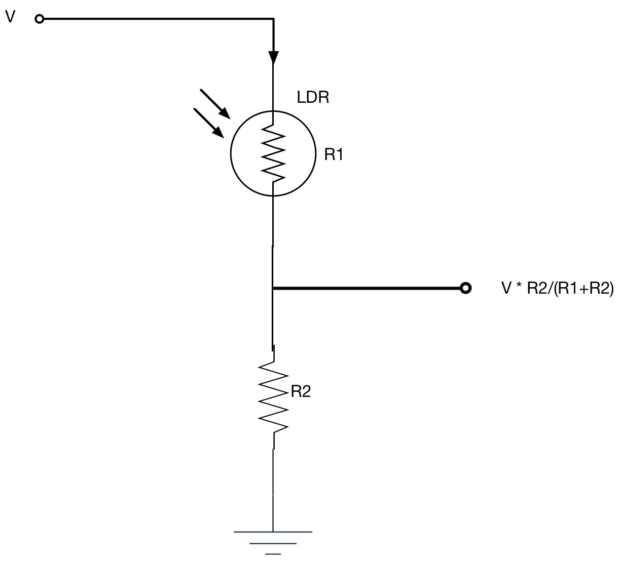
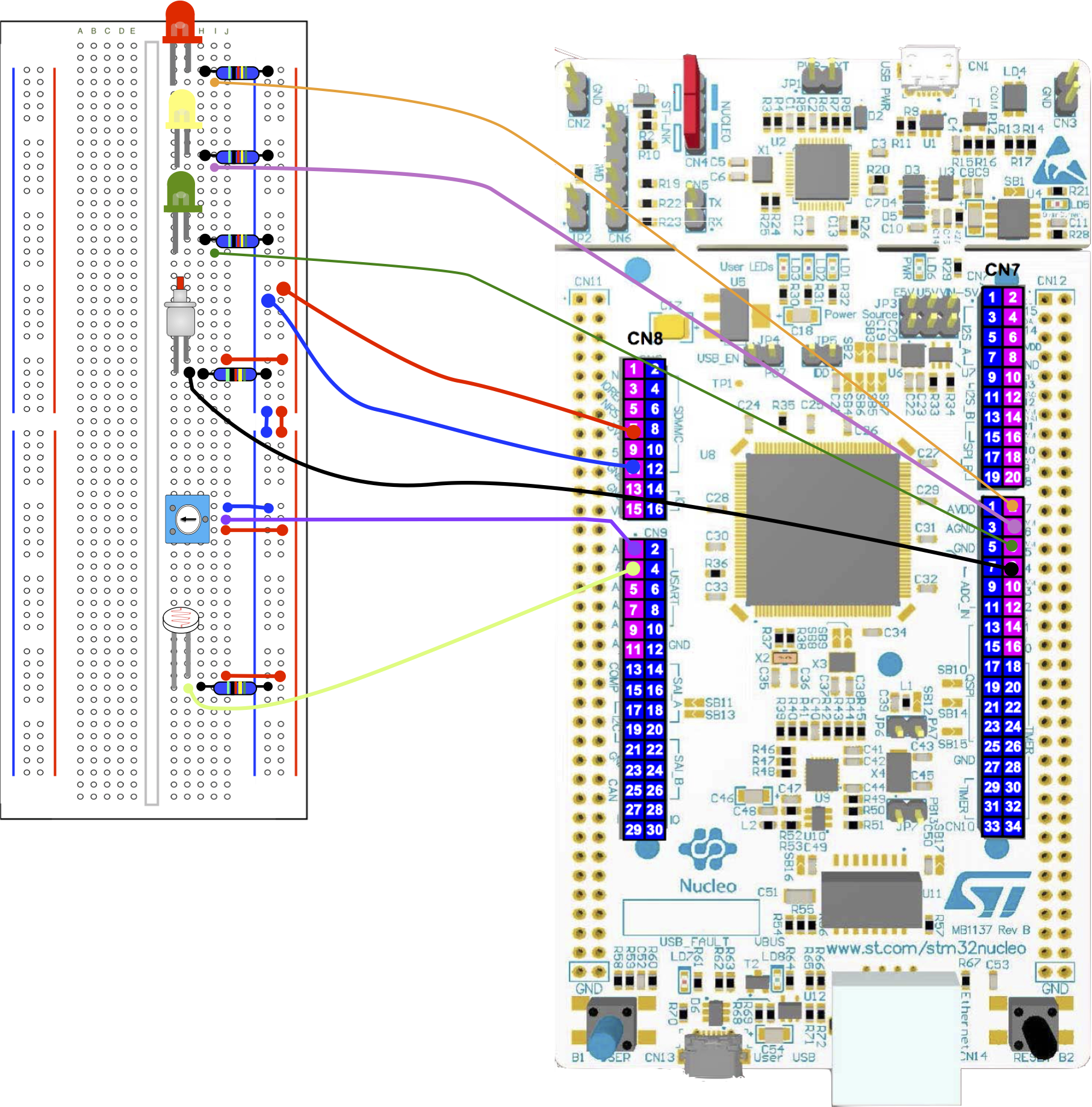
Add the additional circuit below to your existing design (see further down the page for a full prototyping layout)

Create a new project, build and run the sample code below

Run PuTTY, and observe the outputs of this code in the terminal screen. Try rotating the potentiometer and blocking light from the LDR.

Set the potentiometer such that when you move your hand over the LDR, so the LED’s switch ON (See video below)

https://www.youtube.com/watch?v=lCB5O5XBR-k

Using an LDR within a potential divider circuit to generate a light dependent voltage.

#include "mbed.h"

#define kRED    (1 << 2)    //4
#define kYELLOW (1 << 1)    //2
#define kGREEN  (1 << 0)    //1
#define kALL (kRED | kYELLOW | kGREEN)

//Global objects
BusOut binaryOutput(D5, D6, D7);
DigitalIn SW1(D3);
DigitalIn SW2(D4);

AnalogIn POT_ADC_In(A0);
AnalogIn LDD_ADC_In(A1);
float fPOT, fLDR = 0.0;

//Main function
int main() {
   
   while(1) {
      
      //Read ADC
      fPOT = POT_ADC_In;
      fLDR = LDD_ADC_In;
      
      //Write to terminal
      printf("POT = %6.4f\tLDR = %6.4f\n", fPOT, fLDR);
      
      if (fLDR > fPOT) {
         binaryOutput = 0;      //Binary 000
      } else {
         binaryOutput = kALL;   //Binary 111
      }
      
      //Wait
      wait(0.1);
      
   } //end while(1)
} //end main

Wiring instructions for the Light Dependent Resistor (LDR)

Task 4.2.2

Perform the following tasks:

Now watch the video below

Using if and else-if statements, modify your code to achieve this. You can see a solution here.

https://youtube.com/watch?v=aum8M_211uE

Activity 4.3 Noise and Averaging

Watch the following video to observe the analogue signal generated by the LDR.

https://youtube.com/watch?v=ze2TYUZUKlQ

As you can clearly see, the signal is not a smooth line, but has noise superimposed upon it.

In this next activity, we are going to calculate an average of the input signal. We assume the noise is a “random signal” which over time, will average to a value close to zero.

Let us assume the measured signal can be described by as follows:

$y(t) = s(t) + n(t)$

where $y(t)$ is the measured signal we observe (measured in Volts), $s(t)$ is the perfect noise-free signal we want to observe, $n(t)$ is the noise and $t$ is time (in seconds).

We assume the noise $n(t)$ is a random signal with a mean of zero.
As $s(t)$ is a function of light intensity, we can assume this changes very slowly. Over short periods, we can approximate it to be a constant. It is not random.

We can therefore do the following:

$average \{ y(t) \} = average \{ s(t) + n(t) \}$

Written formally:

$E \{ y(t) \} = E \{ s(t) + n(t) \}}$

where $E{\cdot}$ represents the “expected value”, or “average value” in our case.

Without going into too much mathematics, because the function $E{\cdot}$ is linear, so we can also say:

$E \{ y(t) \} = E \{ s(t) + n(t) \} = E \{ s(t) \} + E \{ n(t) \}$

We can use our first assumption:

We say that “in the limit”, as $t \rightarrow \infty$ then $E \{ n(t) \} \rightarrow 0$

$\therefore E \{ y(t) \} \approx E \{ s(t) \}$

In other words, if we measure the average of the noisy signal, then we should begin to estimate the average of the signal itself. We now apply our second assumption:

Over a short time period, we can approximate our signal $s(t)$ to be constant such that $s(t) \approx E \{ s(t) \}$

In other words, if we calculate the average input signal, we can estimate its true value. The longer time used for the average, the more noise will be removed, however this assumes the signal does not change. Let’s now do this in code.

The average of a signal is estimated by measuring and summing N input samples, then dividing the total by N.

Mathematically we write this as:

$E \{ y(n) \} = \frac{1}{N} \cdot \sum_{n=0}^{N-1} x(n)$

$x(n)$ is the $n^{th}$ input signal and $n$ is the sample number. This mathematical expression translates as:

Sum N samples $n(n)$ , where $n=0 ... (N-1)$ , then divide by $N$ .

If we sample the signal 100 times a second, we say the sampling rate $F_s=100Hz$ and the time period $T=\frac{1}{F_s}=0.01s$ .

Don’t worry if you struggle to follow the mathematics above. Much of the problem often stems fro understanding the notation which becomes more familiar with time and practise.

Task 4.3.1

Perform the following tasks:

For both analogue inputs, modify the code below to calculate the average of N=10 samples. Samples should be recorded 100 times a second

Use the printf function to output the average of both potentiometer and LDR signals

Use the provided flowchart to guide you.

#include "mbed.h"

//Global objects
BusOut binaryOutput(D5, D6, D7);
AnalogIn POT_ADC_In(A0);
AnalogIn LDD_ADC_In(A1);

float fPOT, fLDR = 0.0;

//Main function
int main() {
   
   while(1) {
      
      //Read ADC
      fPOT = POT_ADC_In;
      fLDR = LDD_ADC_In;
      
      //TODO:
      //Calculate the average of both fPOT and fLDR,
      //then write to the terminal
      
      //Write to terminal
      printf("POT = %6.4f\tLDR = %6.4f\n", fPOT, fLDR);
      
      if (fLDR > fPOT) {
         binaryOutput = 0;      //Binary 000
      } else {
         binaryOutput = 7;   //Binary 111
      }
      
      //Wait 0.01s
      wait(0.01);
      
   } //end while(1)
} //end main

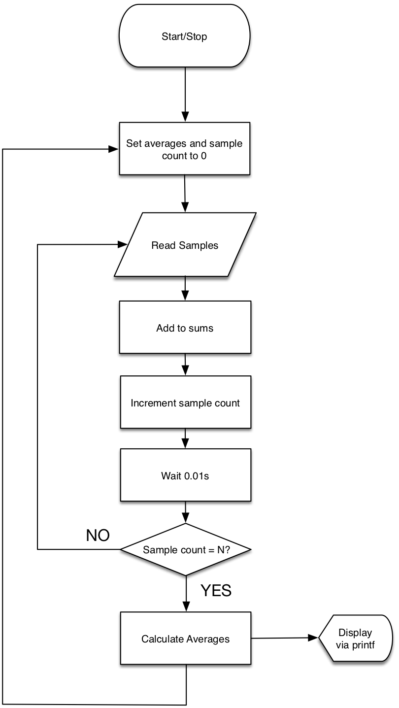
Flowchart for the signal averaging task.

TIP – The input samples are integers. An average is a fractional value. To convert an integer (type int ) to a fractional value (type float ), you can use a type cast.
int x = 10; //Integer variable

float y = (float)x; //Convert x to a float

A solution can be viewed here.

Important Terminology

In task 4.3.1, we measured samples 100 times a second. We say the sampling rate is 100 samples per second. This is also commonly known as 100 Hertz (100Hz), named after the physicist Heinrich Rudolf Hertz. We can also say the sampling interval T = 0.01s (10ms).

Task 4.3.2

Perform the following:

How precise and consistent is the sampling rate in 4.3.1? (hint – remember that lines of code take time to execute).

Using your solution in 4.3.1 (or the solution provided), look at the output in the terminal. Ideally, the averaged value would be constant, however due to noise, there will still be some variation. To how many decimal places is the signal constant?

By increasing N from 10 to 100, estimate to how many decimal places the average signal is constant. How does increasing N impact on the effect of noise? How does it impact on ‘responsiveness’?

Discussion

In terms of precision, the delay of the wait(0.01) statement results in a very precise delay, but the time for the remaining code also needs to be added.

The sampling interval $T = 0.01 + T_{code}$

where $T_{code}$ is the time for remaining code to execute.

In terms of consistency, there is a conditional ( if ) statement in this code. Therefore $T_{code}$ is variable (every N samples, the code branches).

Increasing N will reduce the impact of noise. Note also that increasing N will also reduce responsiveness. You could increase the sampling rate to correct for this, but there are better solutions.

A further problem with our current design is that the output is only updated every N samples. As N becomes large, so the time between measurements also becomes large.

A more elegant solution is to store the past data in an array. Each time a new sample is added, we throw away the oldest sample and recalculate.

There are a number of ways to achieve this, some more efficient than others. Let’s start with the simplest to understand, but most inefficient.

In C or C++, we can create an array of N samples as follows:

float x[8];

In this case, I have created an array of 8 samples to keep the diagrams small. In practice we will use larger arrays. We can visualise an array of samples as a sequence of numbered storage elements as shown below.

The first element of the array is x[0] and the last is x[7] . We can write some code to calculate the average of all elements in the array. For this we will use a for-loop.

int N=8;
float sum = 0;

for (int n=0; n<N; n++) {
   sum += x[n];
}

float average = sum / (float)N;

We can now output the average as required. When we measure the next sample, we can update our array and recalculate as follows.

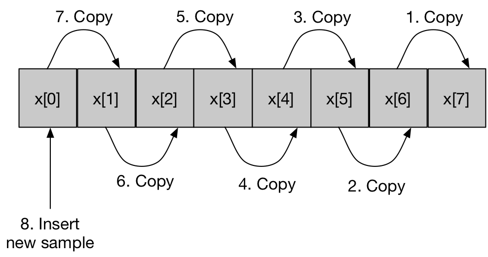
Depicting the logical shifting of elements in an array to create a “First In First Out” (FIFO) buffer.

Note the order of the operations are numbered. First x[6] is copied over the oldest sample x[7] . Then x[5] is copied over x[6] etc.. The last operation is to overwrite x[0] with the newly measured sample. We can now re-calculate the average as before.

It should be noted at this point that the literal copying of samples (as depicted) is not the most efficient technique and that there are faster methods that are logically equivalent.

Task 4.3.3

Perform the following:

Sketch a flow-chart for the method just described

Create a new project and implement this method in code.

Make the array N samples in size, where N is defined as a constant. e.g.

#define N 10

If you get stuck, take a peek at the solution

In what ways do you think this method is inefficient?

Now watch the video (below) on how to log the data for off-line analysis on your PC.

If you wish, repeat this procedure for yourself. It’s a useful technique.

https://youtube.com/watch?v=ojgWI-v5LUw%3Flist%3DPLhsioMrc4CkpVxHnrXO8wjSVWlMTnT6N_

One solution is provided. Note also the following:

The copying of data in the array is both repetitive and inefficient in computation. Instead of moving all the samples in the array, all we really need to do is overwrite the oldest sample and recalculate (this is known as a circular buffer). Furthermore, the average is based on the sum of all elements in the array, we can simply “update” our sum as follows:

$average(n+1)=average(n)+newSample-oldestSample$

Note that I have also created an instance of “Serial ”. This allows data to be written back to the terminal at higher speeds (115200 bits/second), equivalent to 14500 Bytes per second.

You may also have found there was a lot of repetition in your solution (and mine!). Using functions can help reduce repetition and bugs. Consider the following function prototype:

float updateAverage(float newSample, float buffer[]);

This function accepts two parameters. The new sample (a single float) and the buffer (an array of float) used to store past samples.The function returns the average (single float).

Task 4.3.4

Perform the following:

Starting with the code below, complete the function and use it to shorten the code. A solution is provided in case you want to check your answer.

#include "mbed.h"

//Constants
#define N 10

//Function Prototype
float updateAverage(float newSample, float buffer[]);

//Global objects
Serial pc(USBTX, USBRX);

BusOut binaryOutput(D5, D6, D7);
AnalogIn POT_ADC_In(A0);
AnalogIn LDR_ADC_In(A1);

float xPOT[N]; //Aray of potentiometer samples
float xLDR[N]; //Aray of LDR samples

//Main function
int main()
{
   
   //Set baud rate to 115200
   pc.baud(115200);
   
   //Print header
   pc.printf("POT,LDR,avPOT, acLDR\n\n");
   
   while(1) {
      
      //Move the samples in both arrays to the right
      for (unsigned int n=(N-1); n>0; n--) {
         xPOT[n] = xPOT[n-1];
         xLDR[n] = xLDR[n-1];
      }
      
      //Insert the new sample at position 0
      xPOT[0] = POT_ADC_In;
      xLDR[0] = LDR_ADC_In;
      
      //Calculate average for POT
      float fSum = 0.0;
      for (unsigned int n=0; n<N; n++) {
         fSum += xPOT[n];
      }
      float fPOTAverage = fSum / (float)N;
      
      //Calculate average for LDR
      fSum = 0.0;
      for (unsigned int n=0; n<N; n++) {
         fSum += xLDR[n];
      }
      float fLDRAverage = fSum / (float)N;
      
      //Write to terminal via Serial interface
      pc.printf("%6.4f,%6.4f,%6.4f,%6.4f\n", xPOT[N/2], xLDR[N/2], fPOTAverage, fLDRAverage);
      
      //Check the threshold
      if (fLDRAverage > fPOTAverage) {
         binaryOutput = 0;   //Binary 000
      } else {
         binaryOutput = 7;   //Binary 111
      }
      
      //Wait 1/100th second
      wait(0.01);
      
      
   } //end while(1)
} //end main


/*
 First version of the updateAverage function
 TODO
 */
float updateAverage(float newSample, float buffer[])
{
   //Local variable - remember to initialise!
   float average = 0.0;
   
   //TODO: Move all samples to the right
   
   
   //TODO: Insert new sample
   
   
   //TODO: Calculate average
   
   //Return the result
   return average;
}

The sampling rate is still not constant. The time between each sample read depends on the execution time of the code each time around the loop. Not only will this change as the code is maintained, but different “optimisation settings” or even a change in “compiler version” will impact on code execution time.

To address this, we can use a timer interrupt (read the glossary entry to learn more about interrupts).

In Mbed-os, there is a component called a “Ticker ”. This object maintains a hardware timer. When that timer reaches a specified value, it calls the function you specify. This function takes no arguments and returns no data. For example:

void func();

It is probably best to give an example to explain this.

#include "mbed.h"

//Global objects
DigitalOut myled(LED1);
Serial pc(USBTX, USBRX);
Ticker t;

//Integer state of the LED
//static makes it visible only within main.cpp
static int state = 0;

//Function prototype
void doISR();

int main() {
   
   //Initialise
   pc.baud(115200);
   t.attach(doISR, 2);
   myled = 0;
   
   //Main loop
   while(1) {
      
      //Go to sleep and wait for an ISR to wake
      sleep();    //At is says
      
      //At this point, the ISR has run
      
      //Update LED
      myled = state;
      
      //Echo to terminal
      if (state == 0) {
         pc.printf("LED OFF\n");
      } else {
         pc.printf("LED ON\n");
      }
      wait(0.001); //Plenty of time for the serial port to transmit
   }
}

//Note - the ISR is short, and does NOT 
//call functions such as printf 
//(it's actually unsafe to do so)
//Always check a function is "reentrant"
//before calling it
void doISR() {
   //Toggle 0 to 1, or 1 to 0
   state ^= 1;
}

First we create an instance of the Ticker object

Ticker t;

Now we specify what function it shall call, and how often.

t.attach(doISR, 2);

The first parameter is the name of the function. In fact, this is actually the address of the function in program memory, but that is a detail right now. Sometimes you see it written like this:

t.attach(&doISR, 2);

where the prefix & means “address of”. The ticker is actually a timer, which will call the function doISR every 2 seconds. This time is specified as the second parameter specifies (in seconds).

What might surprise you is the first statement in the while loop, which is:

sleep();

This does what it says: puts the CPU into a sleeping mode. Every 2 seconds, the CPU is woken up and the doISR function is called. On inspection, note that all this function does is toggle a variable between
0 and 1.

The code in the while loop can then resume beyond the sleep() function, which is to update the LED output and write to the terminal.

void doISR() { 
  //Toggle 0 to 1, or 1 to 0
  state ^= 1; 
}

The code in the while loop can then resume beyond the sleep() function, which is to update the LED output and write to the terminal. The CPU then returns to the sleep mode until the ticker wakes it again.

Notes:

The interrupt service routine runs once every 2 seconds. The frequency is fixed, and is independent of the code in the main function, compiler settings etc.. We can say that the ISR is “deterministic” (fully predictable in time).
Any data sent to the serial port (e.g. via printf or puts) will generate a sequence of interrupts during communication. A small delay is added to allow all bytes to be transmitted and for all the interrupts to be processed, otherwise the CPU will be brought out of sleep mode prematurely.

Additional Task 4.3.5

If you have time, try the following:

Can you modify the solution in 4.3.4 to use a Ticker

The sampling rate should be precisely 100Hz (T=0.01s)

Keep the ISR as short as possible.

Add a DigitalOut for pin D8.
DigitalOut strobe(D8);

Inside the ISR, you should measure the POT and LDR samples and toggle the D8 pin

If you have access to an Oscilloscope, verify the sampling rate by monitoring pin D8

Even if you cannot do Task 4.3.5, do take a look at the solution and read the comments.

The scope output on D8 is as follows:

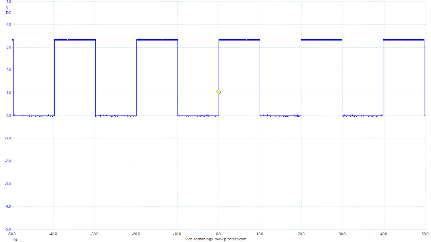
Using an oscilloscope to monitor the output signal on a micro controller pin. Note that signal noise is visible. We can see that the output toggles every 10ms.

The oscilloscope output is shown above. Note the following:

The interval between the signal switching state is measured as 10.0ms which is what was required
The logic ON level is approx. 3.3V and the OFF level is approx. 0V
You can see noise on the signal.

(Digital noise is a reality of life. It can often originate from current spikes and a power supply that is not perfect).

The key point from this exercise is that we can use Timer interrupts to obtain a precise sampling rate. For many applications, this is absolutely critical. Systems that need deterministic timing are often known as real-time systems. Digital Signal Processing (DSP) applications require precise sampling for the mathematics to be valid.

Using interrupts is also more power efficient.

Word of caution. Writing robust (and safe) interrupt code is not trivial, especially as the number of inputs increases. This can lead to problems such as race conditions (data corruption), priority inversion and deadlocks. These topics are beyond the scope of this level 4 course and will be covered in detail elsewhere.

Safer alternatives exist. To manage higher complexity, you might consider using a real-time “operating system” or “real-time micro kernel” to help write complex real-time software. Mbed-os actually offers such a facility, but again, this is beyond the scope of this course (and is covered elsewhere).

Additional Task 4.3.6

Only attempt this if you have time and are confident

If you are feeling ambitious, you can further optimise these solutions (as discussed in the solution of Task 4.3.3). The moving of data in the array is both repetitive and inefficient in computation. Instead of moving all the samples in the array, all we really need to do is overwrite the oldest sample and recalculate. This is known as circular buffering. For this we simply need to keep track of where the oldest and newest sample are stored.

Furthermore, the average is based on the sum of all elements in the array. Instead of calculating the complete sum every time, we can simply “update” our sum as follows:

$average(n+1)=average(n)+newSample-oldestSample$

Improve the solution in 4.3.5 to reduce the computation load using both the methods described

A solution is given here.

Activity 4.4 – Closer look at Analogue to Digital Conversion

We are using the Mbed-os framework (set of objects) to perform rapid development of embedded software. Until now, you have used a DigitalIn object to read the input from an on-chip Analogue to Digital Converter (ADC).

The default behavior is to return a value a fractional value of type float, scaled between 0.0 and 1.0. This is ideal for further processing, but for education, does somewhat mask the true nature of an ADC and the issues around signal conversion.

In this section we delve a little deeper to look at the ADC using some of the other functions in DigitalIn.

Task 4.1.1

Read the glossary entries on Analogue Signals, Digital Signals and the Analogue to Digital Converter

Form a group of 3 from people near you.

Person A will form and ask one or more short questions on a chosen topic

Person B will answer the question verbally for a maximum of 2 minutes

Person C will keep time, observe and give constructive feedback at the end

After each round, rotate roles and topics.

The topics are as follows

Round 1: Analogue Signals

Round 2: Digital Signals

Round 3: Analogue to Digital Conversion

At this point, you probably have a circuit as is shown here. For the next task, ensure you have at least the POT wired.

Task 4.4.2

Perform the following:

Build and run the code below

Monitor the output with PuTTY (Set the rate to 115200)

Turn the POT to discover the minimum and maximum values

Convert the HEX values to decimal

How many bits resolution do you think the ADC has? (8,10, 12t or 16 bit?)

What is the smallest input voltage required to get a value of 1?

#include "mbed.h"

//Function prototype
void doSample1Hz();

//Global objects
Serial pc(USBTX, USBRX);
AnalogIn POT_ADC_In(A0);
DigitalOut led(LED1);

//Shared variables
volatile static unsigned short sample16 = 0;

//The ticker, used to sample data at a fixed rate
Ticker t;

//Main function
int main()
{
   //Set baud rate to 115200
   pc.baud(115200);
   
   //Set up the ticker - 100Hz
   t.attach(doSample1Hz, 1.0);
   
   while(1) {
      
      //Sleep
      sleep();
      
      //Displauy the sample in HEX
      pc.printf("ADC Value: %X\n", sample16);
      
   } //end while(1)
} //end main

//ISR for the ticker - simply there to perform sampling
void doSample1Hz()
{
   //Toggle on board led
   led = !led;
   
   //READ ADC as an unsigned integer.
   //Shift right 4 bits & store in static global variable
   sample16 = POT_ADC_In.read_u16() >> 4;
}

Calculating Logs

To perform a log in a base $B$ , you can use any log function on your calculator:

$log_B(a)=\frac{log(a)}{log(B)}$

For example, for $log_2{16}=\frac{log_{10}(16)}{log_{10}(2)}=4$

Similarly, $log_2{16}=\frac{ln(16)}{ln(2)}=4$

Solution

The range is 000.. FFF (hex), which in decimal is 0..4095. Therefore, there are 4096 possible values.

$log_{2}(4096)= 12$ bits

Given the input range is 0…3.3V, the quantization level $\Delta = \frac{3.3}{4096-1}=0.806mV$

The ADC will output a 1 when the input exceeds $\Delta / 2$

Advanced Task 4.4.3

If you have time, try the following:

Modify the code in task 4.4.2 to write the terminal output in binary format

Hint : use the & operator to test each of the 12 bits. Try and use a for-loop to keep your solution compact and short

A solution is given here.

Advanced Task 4.4.4

Again, if you have time, try the following:

Using only unsigned short and integer arithmetic, calculate the average value of the POT.

Use a sampling rate of 100Hz

Hint: let N be a power of 2, and use a right-shift >> to perform the division.

A solution is given here.

Some words of caution

In this section, we’ve had a first look at interfacing a micro controller to the analogue world. This has hopefully been a useful introduction to the practical mechanisms of sampling analogue signals such that real-world signals can be represented digitally inside a computer. We also had a first look at interrupts.

It is important to note that this is only an introduction.

There is much more to learn when it comes to sampling real-world signals correctly such that they can be properly mathematically analysed and/or processed. This is a topic that will be covered in another course (level 5 onwards).
As mentioned in the text above, interrupts can be hazardous – their asynchronous nature means running code may be interrupted at unpredictable times, and in the absence of protection, can results in data inconsistency or even corruption (known as a race condition). Again, this is a topic that is covered in later stages. For now, the intention is that you are aware of interrupts and understand the very basic concept. It is not recommended that you use interrupts outside of personal experimentation until you know more.

There is a saying, which goes something like this:

A little knowledge is a dangerous thing

or sometimes:

A little learning is a dangerous thing

This is particularly true for topics such as interrupts and analogue to digital conversion.

Back to ToC

Feedback

If you wish to leave feedback or have a question, please use the form below.

[contact-form][contact-field label=”Name” type=”name” required=”true” /][contact-field label=”Email” type=”email” required=”true” /][contact-field label=”Website” type=”url” /][contact-field label=”Message” type=”textarea” /][/contact-form]